Predicting Water Quality with Machine Learning
At Locus Technologies, we’re always looking for innovative ways to help water users better utilize their data. One way we can do that is with powerful technologies such as machine learning. Machine learning is a powerful tool which can be very useful when analyzing environmental data, including water quality, and can form a backbone for competent AI systems which help manage and monitor water. When done correctly, it can even predict the quality of a water system going forward in time. Such a versatile method is a huge asset when analyzing data on the quality of water.
To explore machine learning in water a little bit, we are going to use some groundwater data collected from Locus EIM, which can be loaded into Locus Platform with our API. Using this data, which includes various measurements on water quality, such as turbidity, we will build a model to estimate the pH of the water source from various other parameters, to an error of about 1 pH point. For the purpose of this post, we will be building the model in Python, utilizing a Jupyter Notebook environment.
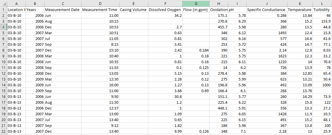
When building a machine learning model, the first thing you need to do is get to know your data a bit. In this case, our EIM water data has 16,114 separate measurements. Plus, each of these measurements has a lot of info, including the Site ID, Location ID, the Field Parameter measured, the Measurement Date and Time, the Field Measurement itself, the Measurement Units, Field Sample ID and Comments, and the Latitude and Longitude. So, we need to do some janitorial work on our data. We can get rid of some columns we don’t need and separate the field measurements based on which specific parameter they measure and the time they were taken. Now, we have a datasheet with the columns Location ID, Year, Measurement Date, Measurement Time, Casing Volume, Dissolved Oxygen, Flow, Oxidation-Reduction Potential, pH, Specific Conductance, Temperature, and Turbidity, where the last eight are the parameters which had been measured. A small section of it is below.

Alright, now our data is better organized, and we can move over to Jupyter Notebook. But we still need to do a bit more maintenance. By looking at the specifics of our data set, we can see one major problem immediately. As shown in the picture below, the Casing Volume parameter has only 6 values. Since so much is missing, this parameter is useless for prediction, and we’ll remove it from the set.

We can check the set and see that some of our measurements have missing data. In fact, 261 of them have no data for pH. To train a model, we need data which has a result for our target, so these rows must be thrown out. Then, our dataset will have a value for pH in every row, but might still have missing values in the other columns. We can deal with these missing values in a number of ways, and it might be worth it to drop columns which are missing too much, like we did with Casing Volume. Luckily, none of our other parameters are, so for this example I filled in empty spaces in the other columns with the average of the other measurements. However, if you do this, it is necessary that you eliminate any major outliers which might skew this average.
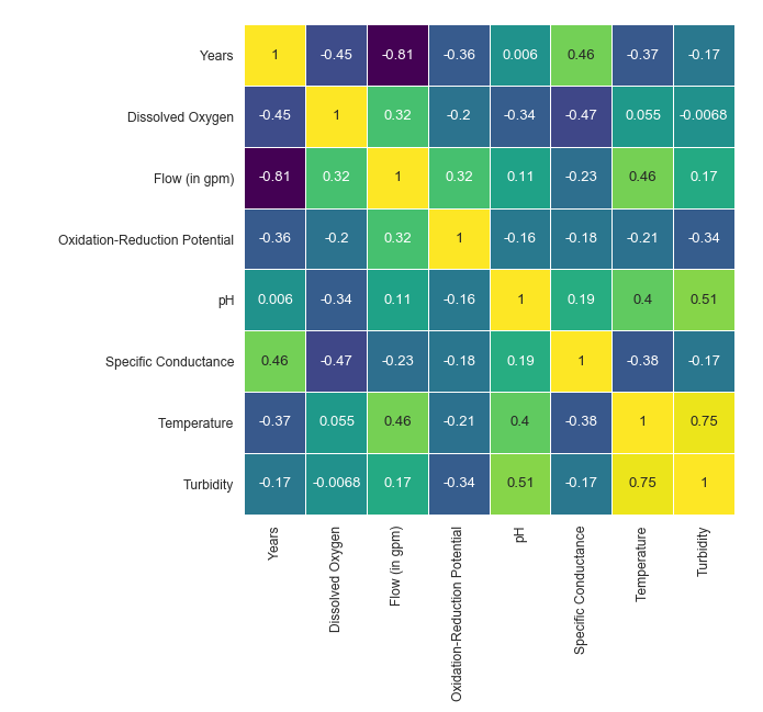
Once your data is usable, then it is time to start building a model! You can start off by creating some helpful graphs, such as a correlation matrix, which can show the relationships between parameters.

For this example, we will build our model with the library Keras. Once the features and targets have been chosen, we can construct a model with code such as this:

This code will create a sequential deep learning model with 4 layers. The first three all have 64 nodes, and of them, the initial two use a rectified linear unit activation function, while the third uses a sigmoid activation function. The fourth layer has a single node and serves as the output.
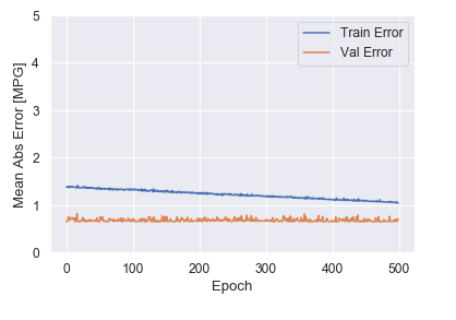
Our model must be trained on the data, which is usually split into training and test sets. In this case, we will put 80% of the data into the training set and 20% into the test set. From the training set, 20% will be used as a validation subset. Then, our model examines the datapoints and the corresponding pH values and develops a solution with a fit. With Keras, you can save a history of the reduction in error throughout the fit for plotting, which can be useful when analyzing results. We can see that for our model, the training error gradually decreases as it learns a relationship between the parameters.

The end result is a trained model which has been tested on the test set and resulted in a certain error. When we ran the code, the test set error value was 1.11. As we are predicting pH, a full point of error could be fairly large, but the precision required of any model will depend on the situation. This error could be improved through modifying the model itself, for example by adjusting the learning rate or restructuring layers.

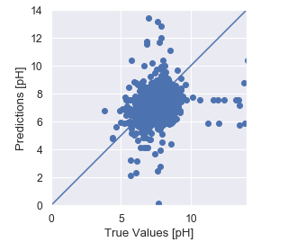
You can also graph the true target values with the model’s predictions, which can help when analyzing where the model can be improved. In our case, pH values in the middle of the range seem fairly accurate, but towards the higher values they become more unreliable.

So what do we do now that we have this model? In a sense, what is the point of machine learning? Well, one of the major strengths of this technology is the predictive capabilities it has. Say that we later acquire some data on a water source without information on the pH value. As long as the rest of the data is intact, we can predict what that value should be. Machine learning can also be incorporated into examination of things such as time series, to forecast a trend of predictions. Overall, machine learning is a very important part of data analytics and the development of powerful AI systems, and its importance will only increase in the future.
What’s next?
As the technology around machine learning and artificial intelligence evolves, Locus will be working to integrate these tools into our EHS software. More accurate predictions will lead to more insightful data, empowering our customers to make better business decisions.
